SpatialAnno

Install the SpatialAnno

This vignette provides an introduction to the R package SpatialAnno, where the function SpatialAnno implements the model SpatialAnno, an efficient and accurate annotation method for spatial transcriptomics datasets, with the capability of effectively leveraging a large number of non-marker genes with “qualitative” information about marker genes, without using a reference dataset. The package can be installed with the command:

library(devtools)

install_github("Shufeyangyi2015310117/SpatialAnno")

The package can be loaded with the command:

library("SpatialAnno")

SpatialAnno for simulated data

Generating the simulated data

We first set the basic parameter. The spatial locations of 3639 spots were taken from DLPFC section 151673. Cell types are assigned with the manually annotations from the original studies. It contains 7 cell types and some “Unknown”. The number of markers for each cell type is set to 4.

set.seed(100)
library(mvtnorm)
library(SingleCellExperiment)
library(splatter)

dlpfc = readRDS(file =   paste0(path.package("SpatialAnno"),"/extdata/151673.rds"))
pos = colData(dlpfc)[,c("row", "col")]
  
n <- dim(dlpfc)[2] # number of spots
p <- 200 ## number of non-markers
y <- as.numeric(colData(dlpfc)[,c("layer_guess_reordered")])
y[is.na(y)] = 8
y2 <- paste0("ct", y)
y2[y2=="ct8"] = "Unknown"
K <- length(table(y)) -1 ## number of clusters
num_mk_per_ct = 5 ## number of markers per cell type
m <- num_mk_per_ct  * K ## number of markers

Then we define the function that can generate raw count. We simulated gene expression for each spot using the splatter package. The parameter for the proportion of DEGs (de.prob) in each layer was set as 0.5. The DE strength is determined by both mean parameter de.facloc and scale parameter de.facScale, the former ranges from 0.1 to 0.8 and the latter was set within [0.1,1], corresponding to the log fold change in expression from one-fold to two-fold across different types. All the other parameters are set based on their estimates in the seven layers from DLPFC section 151673.

generate_count <- function(J = 100, de_facLoc = 0, de_facScale = 1){

  dlpfc = readRDS(file =  paste0(path.package("SpatialAnno"),"/extdata/151673.rds"))
  n <- dim(dlpfc)[2] # number of spots
  p <- 2000 ## number of non-markers
  y <- as.numeric(colData(dlpfc)[,c("layer_guess_reordered")])
  y[is.na(y)] = 8

  dec <- scran::modelGeneVar(dlpfc)
  top <- scran::getTopHVGs(dec, n = 2000)
  cnts = as.matrix(counts(dlpfc)[top,])
  init_params <- splatEstimate(cnts)
  
  num_mk_per_ct = 5
  batch_facLoc = 0
  C = 8
  I = NULL
  N = 7000
  L = 1
  
  de_prop = rep(0.5,8)
  debug = FALSE
  
  # 1.simulate count data
  noBatch <- ifelse(batch_facLoc == 0, TRUE, FALSE)
  group_prob <- as.vector(table(y)/length(y))
  
  
  params <- setParams(
    init_params, 
    batchCells = rep(N, L), # 3N here represents a large number such that
    # we have sufficient cells of each type to be 
    # allocated to the spatial transcriptomics data
    batch.rmEffect = noBatch,
    batch.facLoc = batch_facLoc,
    nGenes = J,
    group.prob = group_prob,
    out.prob = 0,
    de.prob = de_prop,
    de.facLoc = de_facLoc,
    de.facScale = de_facScale)
  
  sim_groups <- splatSimulate(
    params = params, 
    method = "groups", 
    verbose = FALSE)
  
  library(Seurat)
  library(scuttle)
  sim_groups <- logNormCounts(sim_groups)
  seu = as.Seurat(sim_groups)
  seu = SCTransform(seu, assay = "originalexp")
  Idents(seu) = seu@meta.data$Group
  all.markers = FindAllMarkers(seu, assay = "SCT", logfc.threshold = 0.1)
  
  library(dplyr)
  all.markers %>%
    group_by(cluster) %>%
    top_n(n = num_mk_per_ct, wt = avg_log2FC) -> top5
  
  out = list(top5 = top5, sim_groups = sim_groups, all.markers = all.markers)
  return(out)
  
}

generate raw count and marker gene matrix

Five marker genes for each cell type were selected from the top DEGs based on log-fold change.

res1 = generate_count(J = 100, de_facLoc = c(1,2,3,4,5,6,7,8)*0.1, de_facScale = c(0.1,0.1,1,0.1,1,1,0.10,0.1))
res2 = generate_count(J = p, de_facLoc = c(1,2,3,4,5,6,7,8)*0.1, de_facScale = c(0.1,0.1,1,0.1,1,1,0.10,0.1))

res1$all.markers %>%
  group_by(cluster) %>%
  top_n(n = 15, wt = avg_log2FC) -> top15
adjusted_top5_gene = top15$gene[c(1:5,16:20,31:35,46:50,61:65,76:80,91:95)]
##################################1:5,16:20,31:35,46:50,61:65,76:80,91:95
### c(11:15,26:30,31:35,56:60,61:65,86:90,101:105)

## reorder the sample to be matched with y
Groupy = paste0("Group", y)
num_each_celltype = table(y)
idx1 = rep(0, length(y))
for (i in 1:8){
  idx1[y==i] = which(colData(res1$sim_groups)[,3] == paste0("Group",i))[1:num_each_celltype[i]] 
}

idx2 = rep(0, length(y))
for (i in 1:8){
  idx2[y==i] = which(colData(res2$sim_groups)[,3] == paste0("Group",i))[1:num_each_celltype[i]] 
}
  
  
## ordered samples
X1 = counts(res1$sim_groups)[unique(adjusted_top5_gene),idx1]
rownames(X1) = gsub("Gene","mk", rownames(X1))
X2 = counts(res2$sim_groups)[,idx2]
colsum = apply(X2,1,sum)
if (min(colsum) == 0){
  idx_not_equal_zero = which(colsum!=0)
  X2 = X2[idx_not_equal_zero,]
}

  
## generate rho
rho <- matrix(0, dim(X1)[1], K+1)
rownames(rho) <- gsub("Gene","mk", rownames(X1))
colnames(rho)[1:(K+1)] <- paste0("ct", 1:(K+1))
colnames(rho)[K+1] <- "Unknown"
res1_top5_gene = gsub("Gene","mk", adjusted_top5_gene)
for (k in 1:K) {
  rho[res1_top5_gene[((k-1)*num_mk_per_ct + 1):(k*num_mk_per_ct)], k] <- 1
}

## define markers
marker = list()
for (k in 1:K){
  marker[[k]] = rownames(rho)[rho[,k]==1]
  names(marker)[k] = colnames(rho)[k]
}

Then we construct the sce object and perform the normalization on simulated data using function logNormCounts implemented in the R packages scran

# -------------------------------------------------
# make BayesSpace metadata used in BayesSpace
counts <- rbind(X1, X2)
## Make array coordinates - filled rectangle
cdata <- list()
cdata$row <- pos[,1]
cdata$col <- pos[,2]
cdata <- as.data.frame(do.call(cbind, cdata))
cdata$imagerow <- cdata$row
cdata$imagecol <- cdata$col 
## Make SCE
## note: scater::runPCA throws warning on our small sim data, so use prcomp
sce <- SingleCellExperiment(assays=list(counts=counts), colData=cdata)
sce$spatial.cluster <- floor(runif(ncol(sce), 1, 3))

metadata(sce)$BayesSpace.data <- list()
metadata(sce)$BayesSpace.data$platform <- "Visium"
metadata(sce)$BayesSpace.data$is.enhanced <- FALSE

sce <- logNormCounts(sce)
X = as.matrix(t(logcounts(sce)))

Run SpatialAnno on simulated datasets

Then we find the neighborhoods using the function find_neighbors2 implemented in our package SpatialAnno, with specifying the type of platform as Visium, as DLPFC 151673 was sequenced on the platform 10x Genomics Visium. After obtaining the sparse neighborhoods matrix Adj_sp, we can run SpatialAnno with normalized gene expression matrix X, sparse neighborhoods matrix Adj_sp, and a list of markers marker. Note that we choose the initial value from annotation methods scSorter due to low-dimensional non-markers.

Adj_sp = find_neighbors2(sce, platform = "Visium")
fit <- SpatialAnno(X = X, Adj_sp = Adj_sp, marker = marker, initial = "scSorter")

## [1] "mk22" "mk23" "mk38" "mk40" "mk44"
## [1] "mk11" "mk23" "mk38" "mk40" "mk41"
## [1] "mk14" "mk48" "mk56" "mk58" "mk88"
## [1] "mk19" "mk54" "mk55" "mk73" "mk92"
## [1] "mk10" "mk49" "mk61" "mk69" "mk87"
## [1] "mk20" "mk33" "mk34" "mk46" "mk63"
## [1] "mk1"  "mk38" "mk5"  "mk73" "mk93"
## iter = 2, loglik= -1467207.486145, dloglik=0.999317 
## iter = 3, loglik= -1160303.555200, dloglik=0.209176 
## iter = 4, loglik= -1159056.221116, dloglik=0.001075 
## iter = 5, loglik= -1158311.122888, dloglik=0.000643 
## iter = 6, loglik= -1157758.472042, dloglik=0.000477 
## iter = 7, loglik= -1157421.496115, dloglik=0.000291 
## iter = 8, loglik= -1157232.511740, dloglik=0.000163 
## iter = 9, loglik= -1157118.927866, dloglik=0.000098 
## iter = 10, loglik= -1157042.299173, dloglik=0.000066 
## iter = 11, loglik= -1156985.611640, dloglik=0.000049 
## iter = 12, loglik= -1156941.352391, dloglik=0.000038 
## iter = 13, loglik= -1156905.571381, dloglik=0.000031 
## iter = 14, loglik= -1156875.913760, dloglik=0.000026 
## iter = 15, loglik= -1156849.423535, dloglik=0.000023 
## iter = 16, loglik= -1156828.276321, dloglik=0.000018 
## iter = 17, loglik= -1156810.074081, dloglik=0.000016 
## iter = 18, loglik= -1156794.243516, dloglik=0.000014 
## iter = 19, loglik= -1156780.356645, dloglik=0.000012 
## iter = 20, loglik= -1156768.083772, dloglik=0.000011 
## iter = 21, loglik= -1156757.166083, dloglik=0.000009 
## iter = 22, loglik= -1156747.397225, dloglik=0.000008 
## iter = 23, loglik= -1156738.610441, dloglik=0.000008 
## iter = 24, loglik= -1156730.669374, dloglik=0.000007 
## iter = 25, loglik= -1156723.461371, dloglik=0.000006 
## iter = 26, loglik= -1156716.892517, dloglik=0.000006 
## iter = 27, loglik= -1156710.883883, dloglik=0.000005 
## iter = 28, loglik= -1156705.368664, dloglik=0.000005 
## iter = 29, loglik= -1156700.289947, dloglik=0.000004 
## iter = 30, loglik= -1156695.598959, dloglik=0.000004 
## iter = 31, loglik= -1156691.253683, dloglik=0.000004 
## iter = 32, loglik= -1156687.217739, dloglik=0.000003 
## iter = 33, loglik= -1156683.459482, dloglik=0.000003 
## iter = 34, loglik= -1156679.951272, dloglik=0.000003 
## iter = 35, loglik= -1156676.668865, dloglik=0.000003 
## iter = 36, loglik= -1156673.590924, dloglik=0.000003 
## iter = 37, loglik= -1156670.698595, dloglik=0.000003 
## iter = 38, loglik= -1156667.975172, dloglik=0.000002 
## iter = 39, loglik= -1156665.405799, dloglik=0.000002 
## iter = 40, loglik= -1156662.977230, dloglik=0.000002 
## iter = 41, loglik= -1156660.677619, dloglik=0.000002 
## iter = 42, loglik= -1156658.209368, dloglik=0.000002 
## iter = 43, loglik= -1156656.140278, dloglik=0.000002 
## iter = 44, loglik= -1156654.172656, dloglik=0.000002 
## iter = 45, loglik= -1156652.297414, dloglik=0.000002 
## iter = 46, loglik= -1156650.507371, dloglik=0.000002 
## iter = 47, loglik= -1156648.796098, dloglik=0.000001 
## iter = 48, loglik= -1156647.157781, dloglik=0.000001 
## iter = 49, loglik= -1156645.587138, dloglik=0.000001 
## iter = 50, loglik= -1156644.079361, dloglik=0.000001 
## iter = 51, loglik= -1156642.630064, dloglik=0.000001 
## iter = 52, loglik= -1156641.235236, dloglik=0.000001 
## iter = 53, loglik= -1156639.891206, dloglik=0.000001 
## iter = 54, loglik= -1156638.594606, dloglik=0.000001 
## iter = 55, loglik= -1156637.342342, dloglik=0.000001 
## iter = 56, loglik= -1156636.131571, dloglik=0.000001 
## iter = 57, loglik= -1156634.959674, dloglik=0.000001 
## iter = 58, loglik= -1156633.824237, dloglik=0.000001

We demonstrate the output of SpatialAnno, which is a list contains many items. We will explain them one by one in the following part.

str(fit)

## List of 13
##  $ R      : num [1:3639, 1:8] 3.46e-52 1.00 3.74e-23 1.42e-48 1.15e-65 ...
##  $ xi     : num 2.5
##  $ type   : int [1:3639, 1] 3 1 7 3 5 6 7 3 1 6 ...
##  $ alpha_m: num [1:30, 1] 1.83 2.87 2.34 3.33 2.98 ...
##  $ bet_m  : num [1:30, 1:8] 1.4 1.16 2.58 1.5 1.13 ...
##  $ mu_m   : num [1:30, 1:8] 3.23 4.02 4.92 4.83 4.1 ...
##  $ sigma_m: num [1:30, 1] 1.88 1.76 1.76 1.57 1.74 ...
##  $ Ez_u   : num [1:3639, 1:15] 8.2 10.11 13.38 8.06 7.23 ...
##  $ Mu_u   : num [1:8, 1:15] 9.59 5.01 8.23 10.59 7.53 ...
##  $ Sgm_u  : num [1:15, 1:15] 4.017 0.445 2.513 0.983 -3.627 ...
##  $ W_u    : num [1:200, 1:15] 0.0785 -0.0292 0.0496 0.0211 0.0439 ...
##  $ Lam_u  : num [1:200, 1] 0.738 0.833 0.709 0.617 0.971 ...
##  $ loglik : num [1:57] -2.15e+09 -1.47e+06 -1.16e+06 -1.16e+06 -1.16e+06 ...

• ‘R’ the estimator of probability that each spot was assigned to these five cell types or “Unknown”. The order of the cell types is the same as that of cell types in gene marker matrix.
• ‘xi’ the estimator of smooth parameter.
• ‘type’ the predicated cell types for each spot.
• ‘alpha_m’ the estimator of base expression level.
• ‘bet_m’ the estimator of extra expression level.
• ‘mu_m’ the mean of cell types in marker group.
• ‘sigma_m’ the covariance matrix of cell types in marker group.
• ‘Ez_u’ the low-dimensional embedding.
• ‘Mu_u’ the mean of cell types in non-marker group.
• ‘Sgm_u’ the covariance matrix of cell types in non-marker group.
• ‘W_u’ the estimator of factor loading matrix.
• ‘Lam_u’ the variance of error in non-marker group.
• ‘loglik’ the vector of log-likelihood of SpatialAnno.

plot the annotation results

The predictions can be obtained in the following way. Then we can plot the annotation results of SpatialAnno on the original positions using R package ggplot2

prediction = colnames(rho)[fit$type]
print(prediction[1:20])

##  [1] "ct3" "ct1" "ct7" "ct3" "ct5" "ct6" "ct7" "ct3" "ct1" "ct6" "ct7" "ct4"
## [13] "ct5" "ct3" "ct5" "ct3" "ct6" "ct5" "ct1" "ct6"

library(ggplot2)
fit_type = colnames(rho)[fit$type]
pos[,1] = -pos[,1]
dat = data.frame(pos[,1], pos[,2], factor(fit_type))
names(dat)= c("imagerow", "imagecol", "Cell type")

p1 <- ggplot(dat, aes(x=imagerow, y=imagecol, color=`Cell type`)) +
  geom_point(size = 3, alpha = 0.5) +
  theme(axis.text.x = element_blank(),
        axis.text.y = element_blank(),
        axis.title.x = element_blank(),
        axis.title.y = element_blank(),
        panel.grid.major = element_blank(),
        panel.grid.minor = element_blank(),
        panel.border = element_blank(),
        axis.ticks = element_blank())+
  guides(colour = guide_legend(override.aes = list(size = 5)))
p1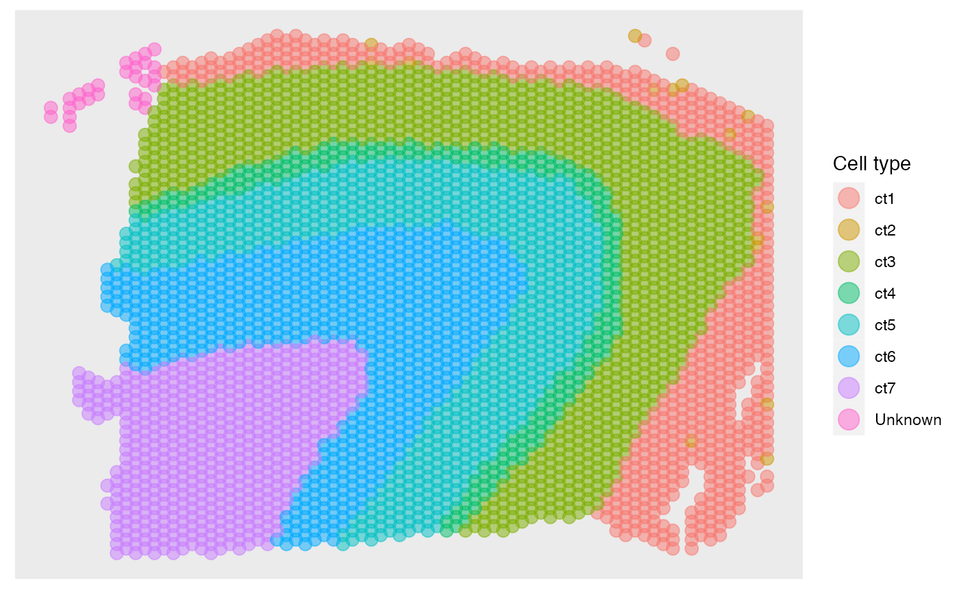

calculate Kappa, mF1, and acc

After obtaining the predictions, we can calculate Kappa, mF1 (mean F1), and acc to evalute the performance of annotation results by SpatialAnno. The function cohen.kappa to calculate Kappa is implemented in the package psych. The function evaluate to calculate mF1 is implemented in our package SpatialAnno. The Kappa is

library(psych)
idx = which(y2!="Unknown" & prediction!="Unknown")
Kappa = cohen.kappa(x = cbind(y2[idx], prediction[idx]))$kappa
print(Kappa)

## [1] 0.9140835

The mF1 is

mF1 = mean(evaluate(y2[idx], prediction[idx])$F1)

print(mF1)

## [1] 0.8183227

The acc is

acc = mean(y2[idx] == prediction[idx])
print(acc)

## [1] 0.9296594

extract the embeddings

Then we extract the embeddings from the output of SpatialAnno, and plot the tSNE and calculate ARI with the function adjustedRandIndex implemented in the R package mclust

library(scater)
embedding = fit$Ez_u
print(head(embedding))

##           [,1]     [,2]      [,3]     [,4]      [,5]       [,6]      [,7]
## [1,]  8.200934 4.476067 11.438057 4.497795 -14.71717  2.2841504  4.460064
## [2,] 10.114228 2.842798 13.357539 4.504574 -14.94004  2.7476946 10.643506
## [3,] 13.383633 2.318947 10.986487 4.481825 -15.31096  1.8013694  7.769313
## [4,]  8.064062 3.235666 10.708896 4.696581 -12.87674  3.0176053  4.083591
## [5,]  7.234133 1.561023  9.402078 4.409085 -14.87095  7.3525165  9.731576
## [6,]  6.485527 2.379345 13.300804 5.590139 -12.80716 -0.9256822  4.942769
##           [,8]       [,9]      [,10]      [,11]     [,12]      [,13]     [,14]
## [1,] -18.60973 -0.4446807 -1.3097434  1.0922510  5.741625 -16.821980 -9.101355
## [2,] -25.92402 -0.7540642 -0.3209393  2.2472831  2.485593  -8.610126 -4.234882
## [3,] -29.58129 -7.8842991  0.6316807 -0.8186432  3.486277  -9.289701 -6.595325
## [4,] -16.73786 -0.5455508 -1.0143665  0.3906326  2.974831 -17.350978 -6.723654
## [5,] -21.72303  1.6026990 -7.1421597 -7.9475153  3.997371  -4.172060 -4.402423
## [6,] -19.11774 -5.3660077 -8.2743829  5.6032033 -2.765648  -3.087866 -5.903869
##           [,15]
## [1,] -4.5227073
## [2,] -3.9502406
## [3,] -3.4842198
## [4,] -2.7758946
## [5,] -0.8484403
## [6,] -2.0439957

tsne = calculateTSNE(t(as.matrix(embedding)))

The tSNE plot is

dat = as.data.frame(tsne)
colnames(dat) = c("X", "Y")
dat$cluster = prediction
library(ggplot2)
p1 <- ggplot(dat, aes(x=X, y=Y, color=cluster)) +
  geom_point(size = 1, alpha = 0.5) +
  theme(axis.text.x = element_blank(),
        axis.text.y = element_blank(),
        axis.title.x = element_blank(),
        axis.title.y = element_blank(),
        panel.grid.major = element_blank(),
        panel.grid.minor = element_blank(),
        panel.border = element_blank(),
        axis.ticks = element_blank())+
  guides(colour = guide_legend(override.aes = list(size = 5), ncol=1))
p1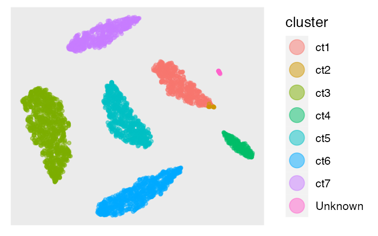

Then we perform the clustering analysis with GMM on embedding and calculate ARI. The ARI is

fit2 = Mclust(embedding, G = 3:10)
ARI = adjustedRandIndex(y, fit2$classification)
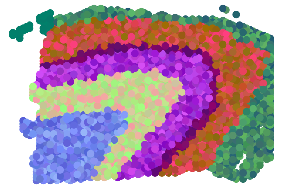
print(ARI)

## [1] 0.6971748

We can also plot RGB plot with the function plot_RGB implemented in PRECAST. The RGB plot is demonstrated as follows

library(PRECAST)
tsne3dim = calculateTSNE(t(embedding), ncomponents = 3)
pList <- plot_RGB(pos, tsne3dim, pointsize = 2)
pList