SC-MEB: installation and simulation

Install the SC.MEB

This vignette provides an introduction to the R package SC.MEB, where the function SC.MEB implements the model SC-MEB, spatial clustering with hidden Markov random field using empirical Bayes. The package can be installed with the command:

library(devtools)

install_github("Shufeyangyi2015310117/SC.MEB")

The package can be loaded with the command:

library("SC.MEB")
#> Loading required package: mclust
#> Warning: package 'mclust' was built under R version 4.0.5
#> Package 'mclust' version 5.4.7
#> Type 'citation("mclust")' for citing this R package in publications.

Fit SC-MEB using simulated data

Generating the simulated data

We first set the basic parameter:

library(mvtnorm)
library(GiRaF)
library(SingleCellExperiment)
set.seed(100)
G <- 4
Bet <- 1
KK <- 5
p <- 15
mu <- matrix(c( c(-6, rep(-1.5, 14)),
               rep(0, 15),
               c(6, rep(1.5, 14)),
               c(rep(-1.5, 7), rep(1.5, 7), 6),
               c(rep(1.5, 7), rep(-1.5, 7), -6)), ncol = KK)
height <- 70
width <- 70
n <- height * width # # of cell in each indviduals

Then, we generate the true clustering label, 15-dimensional PCA and position of each spot.

X <- sampler.mrf(iter = n, sampler = "Gibbs", h = height, w = width, ncolors = KK, nei = G, param = Bet,initialise = FALSE, view = TRUE)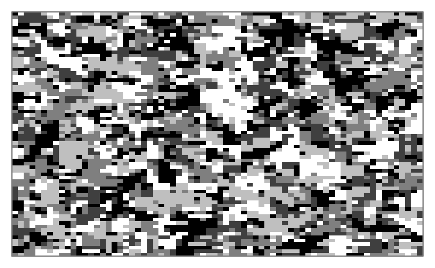

x <- c(X) + 1
y <- matrix(0, nrow = n, ncol = p)

for(i in 1:n)   { # cell
  mu_i <- mu[, x[i]]
  Sigma_i <- ((x[i]==1)*2 + (x[i]==2)*2.5 + (x[i]==3)*3 +
                (x[i]==4)*3.5 + (x[i]==5)*4)*diag(1, p)*0.3
  y[i, ] <- rmvnorm(1, mu_i, Sigma_i)
}

pos <- cbind(rep(1:height, width), rep(1:height, each=width))

Subsequently, we construct the SingleCellExperiment object based on the above PCA and position.

# -------------------------------------------------
# make SC-MEB metadata used in SC-MEB
counts <- t(y)
rownames(counts) <- paste0("gene_", seq_len(p))
colnames(counts) <- paste0("spot_", seq_len(n))

## Make array coordinates - filled rectangle
cdata <- list()
nrow <- height; ncol <- width
cdata$row <- rep(seq_len(nrow), each=ncol)
cdata$col <- rep(seq_len(ncol), nrow)
cdata <- as.data.frame(do.call(cbind, cdata))
## Scale and jitter image coordinates
#scale.factor <- rnorm(1, 8);  n_spots <- n
#cdata$imagerow <- scale.factor * cdata$row + rnorm(n_spots)
#cdata$imagecol <- scale.factor * cdata$col + rnorm(n_spots)
cdata$imagerow <- cdata$row
cdata$imagecol <- cdata$col
## Make SCE
## note: scater::runPCA throws warning on our small sim data, so use prcomp
sce <- SingleCellExperiment(assays=list(counts=counts), colData=cdata)
reducedDim(sce, "PCA") <- y
# sce$spatial.cluster <- floor(runif(ncol(sce), 1, 3))

metadata(sce)$SCMEB.data <- list()
metadata(sce)$SCMEB.data$platform <- "ST"
metadata(sce)$SCMEB.data$is.enhanced <- FALSE

Fitting the SC-MEB

Here, we set the basic paramters for our function SC.MEB

platform = "ST"
beta_grid = seq(0,4,0.2)
K_set= 2:10
parallel=TRUE
num_core = 3
PX = TRUE
maxIter_ICM = 10
maxIter = 50

Here, we briefly explain these parameters.

‘parallel’ is a logical value specifing the run the model in parallel. The default is TRUE.

‘num_core’ is a interger value for the number of cores used for parallel. The default is 5.

‘PX’ is a logical value for paramter expansion in EM algorithm. The default is True.

‘K_set’ is an integer vector specifying the numbers of mixture components (clusters) for which the BIC is to be calculated. The default is K = 2:10.

‘platform’ is the name of spatial transcriptomic platform. Specify ‘Visium’ for hex lattice geometry or ‘ST’ for square lattice geometry. Specifying this parameter is optional as this information is included in their metadata.

‘beta_grid’ is a numeric vector specifying the smoothness of Random Markov Field. The default is seq(0,5,0.2).

‘maxIter_ICM’ is the maximum iteration of ICM algorithm. The default is 10.

‘maxIter’ is the maximum iteration of EM algorithm. The default is 50.

Calculating the neighborhood

First, we require to find the neighborhood

Adj_sp <- getneighborhood_fast(as.matrix(pos), cutoff = 1.2)

Adj_sp <- find_neighbors2(sce, platform = platform)
Adj_sp[1:10,1:10]
#> 10 x 10 sparse Matrix of class "dgCMatrix"
#>                          
#>  [1,] . 1 . . . . . . . .
#>  [2,] 1 . 1 . . . . . . .
#>  [3,] . 1 . 1 . . . . . .
#>  [4,] . . 1 . 1 . . . . .
#>  [5,] . . . 1 . 1 . . . .
#>  [6,] . . . . 1 . 1 . . .
#>  [7,] . . . . . 1 . 1 . .
#>  [8,] . . . . . . 1 . 1 .
#>  [9,] . . . . . . . 1 . 1
#> [10,] . . . . . . . . 1 .

The output ‘Adj_sp’ is a sparse matrix to describe the neighorhood. There two functions are both used to calculate the nrighborhood. The first function ‘getneighobrhood_fast’ is a general function used for general data. However, the second function ‘find_neighbors2’ is a specific function for ST and Visium data.

Run the SC-MEB in parallel

Finally, we run our model SC-MEB by the function SC.MEB.

fit = SC.MEB(y, Adj_sp, beta_grid = beta_grid, K_set= K_set, parallel=parallel, num_core = num_core, PX = PX, maxIter_ICM=maxIter_ICM, maxIter=maxIter)
#> Starting parallel computing...
str(fit[,1])
#> List of 9
#>  $ x     : num [1:4900, 1] 1 1 1 1 1 1 1 1 1 1 ...
#>  $ gam   : num [1:4900, 1:2] 1 1 1 1 1 1 1 1 1 1 ...
#>  $ pxgn  : num [1:4900, 1:2] 0.5 0.668 0.891 0.891 0.891 ...
#>  $ pygx  : num [1:4900, 1:2] 19 22.6 23 30.2 26.1 ...
#>  $ mu    : num [1:15, 1:2] 1.344 0.32 0.352 0.339 0.321 ...
#>  $ sigma : num [1:15, 1:15, 1:2] 8.74 2.84 2.8 2.9 2.88 ...
#>  $ beta  : num 1.4
#>  $ ell   : num 109003
#>  $ loglik: num [1:4, 1] 111455 110576 110167 110167

Here, We briefly explain the output of the SC.MEB.

The item ‘x’ is clustering label.

The item ‘ell’ is the opposite log-likelihood for each beta and K.

The item ‘mu’ is the mean of each component.

The item ‘sigma’ is the variance of each component.

The item ‘gam’ is the posterior probability.

The item ‘beta’ is the estimated smoothing parameter.

Clustering

Selecting the number of clusters using BIC

selectKPlot(fit, K_set = K_set, criterion = "BIC")

Selecting the number of clusters using Modified BIC

Here we briefly explain how to choose the parameter c in the modified BIC. In general, For the ST or Visium dataset, it often ranges from 0.4 to 1 while for the MERFISH dataset with large number of cells, it often becomes larger, for example 10,20. Most importantly, SC-MEB is fast, scaling well in terms of sample size, which allow the user to tune the c based on their prior knowledge about the tissues or cells.

selectKPlot(fit, K_set = K_set, criterion = "MBIC")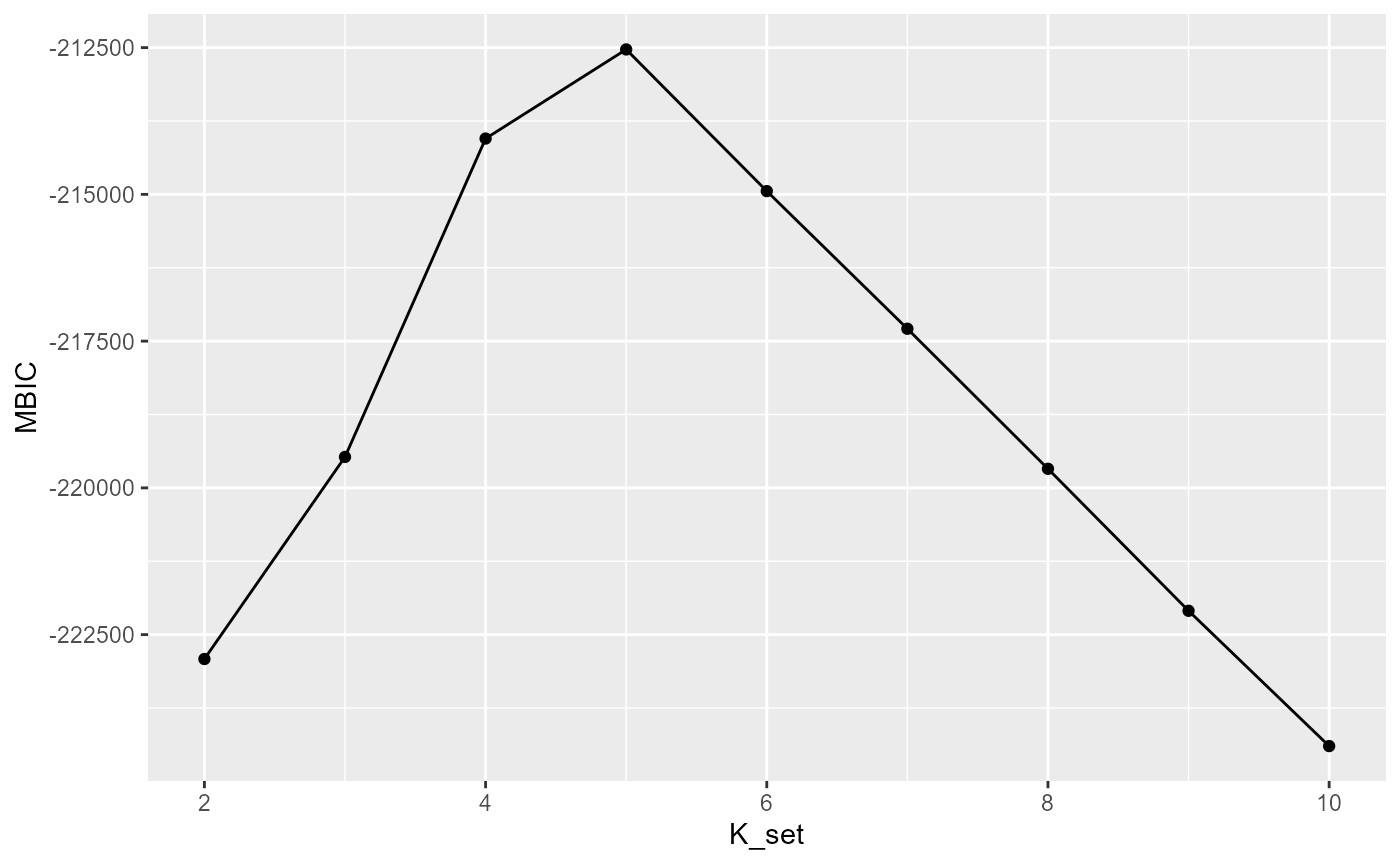

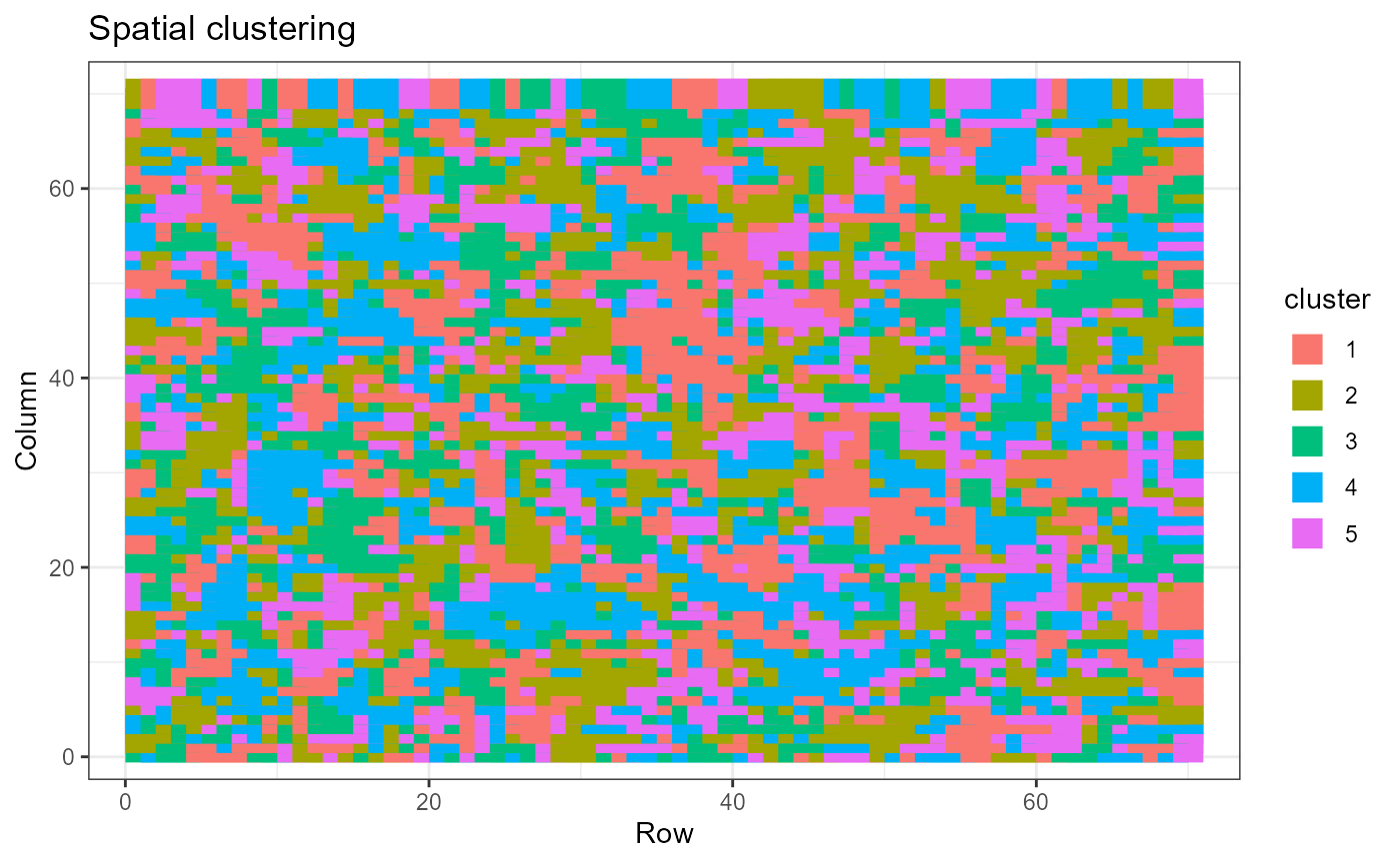
Visualizing spatial clusters

We can plot the cluster assignments over the spatial locations of the spots with ClusterPlot().

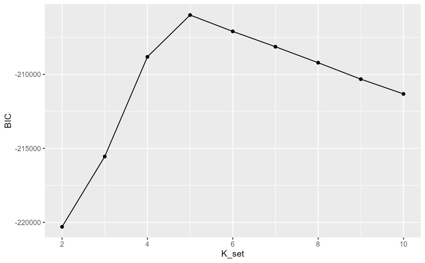
out = selectK(fit, K_set = K_set, criterion = "BIC")
ClusterPlot(out, pos)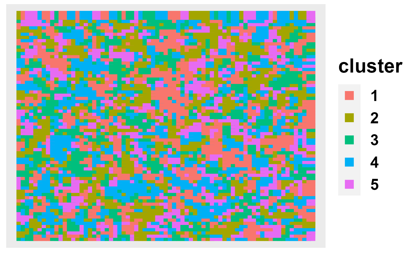

As ClusterPlot() returns a ggplot object, it can be customized by composing with familiar ggplot2 functions.

ClusterPlot(out, pos) +
theme_bw() +
xlab("Row") +
ylab("Column") +
labs(title="Spatial clustering")

Yi Yang

2021-09-02