SC-MEB: CRC
Yi Yang
2021-09-02
SC.MEB_CRC.RmdThe package can be loaded with the command:
library("SC.MEB")
#> Loading required package: mclust
#> Warning: package 'mclust' was built under R version 4.0.5
#> Package 'mclust' version 5.4.7
#> Type 'citation("mclust")' for citing this R package in publications.
Fit SC-MEB using real data CRC
file = system.file("extdata", "CRC3.rds", package = "SC.MEB")
CRC = readRDS(file)
Pre-processing data
SC-MEB requires minimal data pre-processing, but we provide a helper function to automate it.
spatialPreprocess() log-normalizes the count matrix and performs PCA on the top n.HVGs highly variable genes, keeping the top n.PCs principal components. Additionally, the spatial sequencing platform is added as metadata in the SingleCellExperiment for downstream analyses. If you do not wish to rerun PCA, running spatialPreprocess() with the flag skip.PCA=TRUE will only add the metadata SC-MEB requires.
set.seed(114)
library(scuttle)
library(scran)
library(scater)
library(BiocSingular)
CRC <- spatialPreprocess(CRC, platform="Visium")
Here, we set the basic paramters for our function SC.MEB
platform = "Visium"
beta_grid = seq(0,4,0.2)
K_set= 2:10
parallel=TRUE
num_core = 3
PX = TRUE
maxIter_ICM = 10
maxIter = 50
Fitting the SC-MEB
Calculating the neighborhood
library(SingleCellExperiment)
Adj_sp  <- find_neighbors2(CRC, platform = "Visium")
Adj_sp[1:10,1:10]
#> 10 x 10 sparse Matrix of class "dgCMatrix"
#>
#>  [1,] . 1 1 . . . . . . .
#>  [2,] 1 . 1 1 . . . . . .
#>  [3,] 1 1 . 1 1 . . . . .
#>  [4,] . 1 1 . 1 1 . . . .
#>  [5,] . . 1 1 . 1 1 . . .
#>  [6,] . . . 1 1 . 1 1 . .
#>  [7,] . . . . 1 1 . 1 1 .
#>  [8,] . . . . . 1 1 . 1 1
#>  [9,] . . . . . . 1 1 . 1
#> [10,] . . . . . . . 1 1 .
Run the SC-MEB in parallel
y = reducedDim(CRC, "PCA")[,1:15]
fit = SC.MEB(y, Adj_sp, beta_grid = beta_grid, K_set= K_set, parallel=parallel, num_core = num_core, PX = PX, maxIter_ICM=maxIter_ICM, maxIter=maxIter)
#> Starting parallel computing...
str(fit[,1])
#> List of 9
#>  $ x     : num [1:2988, 1] 1 1 1 1 1 1 1 1 1 1 ...
#>  $ gam   : num [1:2988, 1:2] 1 1 1 1 1 ...
#>  $ pxgn  : num [1:2988, 1:2] 0.9 0.996 0.988 0.999 0.988 ...
#>  $ pygx  : num [1:2988, 1:2] 17.6 17.9 29.8 33.4 24 ...
#>  $ mu    : num [1:15, 1:2] 4.3905 -0.5647 0.1235 0.1118 -0.0293 ...
#>  $ sigma : num [1:15, 1:15, 1:2] 5.14 -1.8006 -1.6301 -0.0896 1.0888 ...
#>  $ beta  : num 2.2
#>  $ ell   : num 65515
#>  $ loglik: num [1:2, 1] 66215 66254
Clustering
Selecting the number of clusters using Modified BIC
Here we briefly explain how to choose the parameter c in the modified BIC. In general, For the ST or Visium dataset, it often ranges from 0.4 to 1 while for the MERFISH dataset with large number of cells, it often becomes larger, for example 10,20. Most importantly, SC-MEB is fast, scaling well in terms of sample size, which allow the user to tune the c based on their prior knowledge about the tissues or cells.
selectKPlot(fit, K_set = K_set, criterion = "MBIC")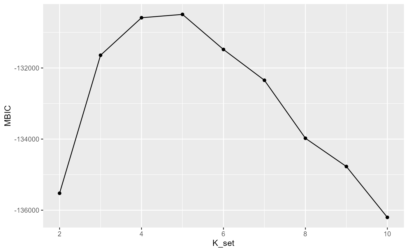
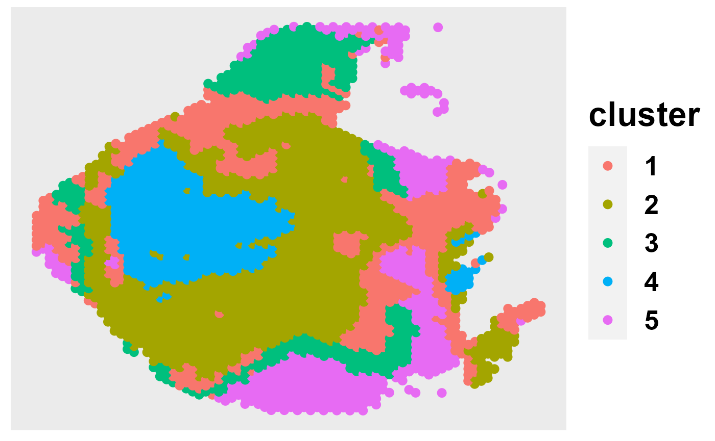
Visualizing spatial clusters
We can plot the cluster assignments over the spatial locations of the spots with ClusterPlot().
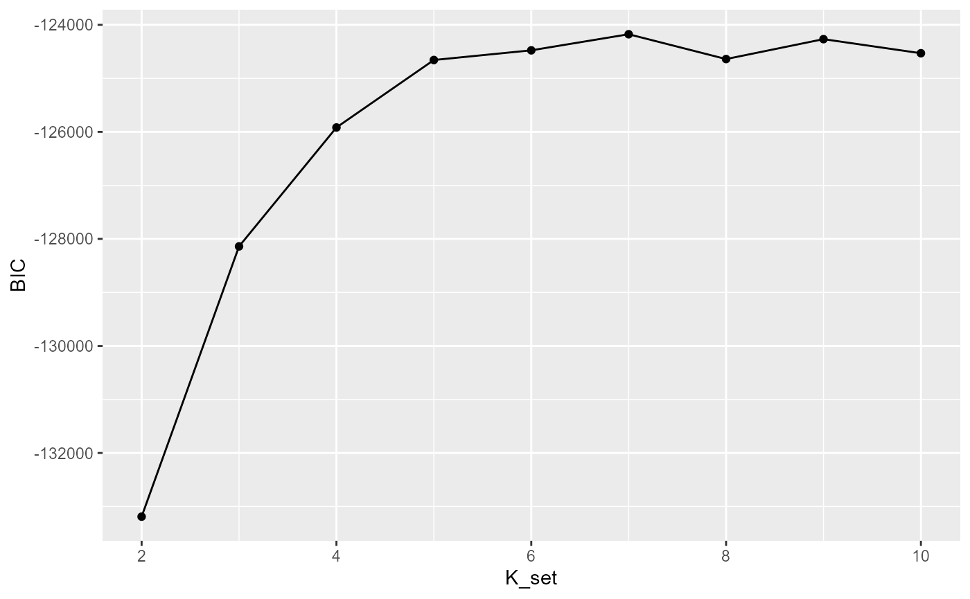
out = selectK(fit, K_set = K_set, criterion = "BIC")
pos = matrix(cbind(colData(CRC)[,c(4)],20000-colData(CRC)[,c(3)]), 2988, 2)
ClusterPlot(out, pos, size = 3, shape = 16)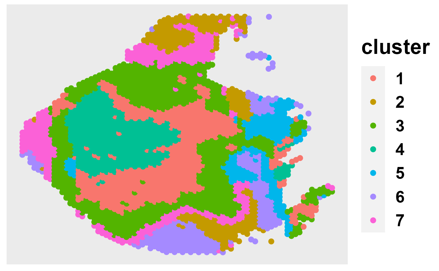 or
or
out = selectK(fit, K_set = K_set, criterion = "MBIC")
pos = matrix(cbind(colData(CRC)[,c(4)],20000-colData(CRC)[,c(3)]), 2988, 2)
ClusterPlot(out, pos, size = 3, shape = 16)